Executive summary
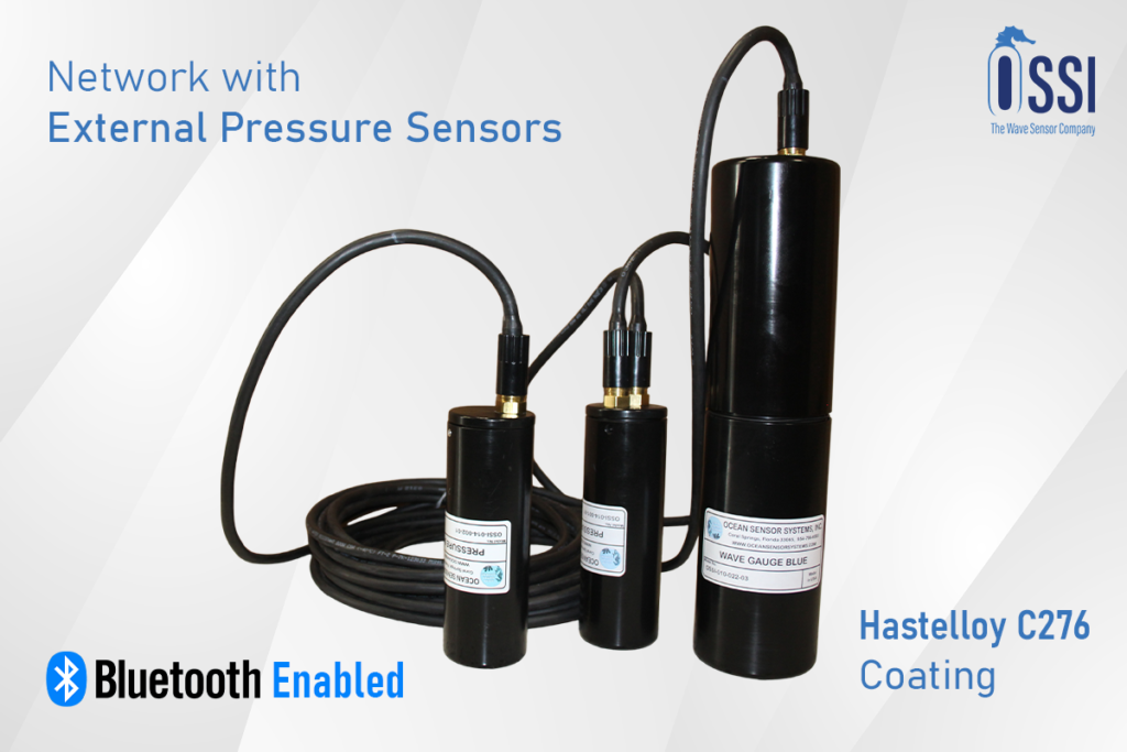
The Wave Gauge Blue (OSSI-010-022) is best understood as a compact, autonomous subsea wave-and-water-level measurement platform rather than merely a generic pressure logger. In a single waterproof housing it combines an absolute pressure transducer, internal logging electronics, removable CompactFlash storage, battery power, and local or shore-linked communications. The official documentation positions it for waves, wakes, tides, sinkage, lake, pond, tank, and pool level monitoring, while the uploaded project notes correctly push the framing further toward real deployment practice and broader engineering applications rather than datasheet-only description.
Technically, the platform is strong where autonomous subsea logging matters most: pressure ranges of 0–1 bar, 0–3 bar, and 0–10 bar; programmable sampling from 2 Hz to 32 Hz in either continuous or burst mode; FAT16/FAT32 CompactFlash support up to 64 GB; a real-time clock specified at ±2 ppm from 0 to 40 °C; and communications through RS232, Bluetooth, and optional RS422/RS485 shore connection. Manufacturer figures give nominal battery endurance of about 2.0 months continuous with the standard 18 V pack and 4.7 months with the extended 21 V pack when Bluetooth is off, rising to 10.3 months and 24.0 months respectively at a 10 % sampling duty cycle. The same platform can also scale to an internal-plus-external array of up to 16 pressure sensors total, subject to the stated sample-rate trade-off.
The engineering value is therefore clear. For remote coastal programmes, reef observatories, harbour studies, offshore structure monitoring, and laboratory hydraulic work, Wave Gauge Blue offers a rare combination of long unattended endurance, simple data recovery, practical field handling, and enough processing support to derive surface-elevation spectra and standard bulk parameters such as Hs/Hm0, Tp, and Hrms from seabed pressure records. Real deployments documented in the literature and observatory practice show exactly that pattern of use, from long-term reef measurements in the South Pacific to dense cross-shore coastal monitoring campaigns in Saint-Malo.
Instrument profile and engineering significance
Wave Gauge Blue combines a temperature-compensated, highly stable pressure sensor, flash-card data logging, internal battery power, and a rugged waterproof ABS housing with a flush Hastelloy diaphragm. The manufacturer describes the instrument as self-logging and self-powered, with standard pressure ranges of 1 bar, 3 bar, and 10 bar, optional external pressure sensors, optional shore connection, and optional water temperature measurement. The user manual further clarifies that the pressure transducer is an absolute transducer zeroed at one atmosphere, so practical gauge pressure is obtained from total pressure minus atmospheric pressure.
| Attribute | Wave Gauge Blue engineering detail |
|---|---|
| Pressure ranges | 0–1 bar, 0–3 bar, 0–10 bar; official ordering variants also available with extended-case battery option |
| Pressure accuracy | ±0.05 % full scale, typical over 10–40 °C; ±0.1 % full scale over −10 to 65 °C |
| Resolution | 0.0033 % of full scale |
| Long-term stability | 0.0005 bar for the 0–1 bar model; 0.05 % FS for the 0–3 bar and 0–10 bar models |
| Construction | Flush Hastelloy diaphragm, ABS housing, Buna-N O-rings, stainless-steel-compatible wetted system |
| Operating temperature | −10 to 65 °C |
| Sampling | Continuous or burst; programmable 2, 4, 8, 16, or 32 Hz |
| Storage | CompactFlash, FAT16/FAT32, 64 MB to 64 GB; ASCII output with time/date and configuration header |
| Timing | Real-time clock accuracy ±2 ppm from 0 to 40 °C |
| Interfaces | Internal RS232, Bluetooth serial connection, optional external-power shore serial link via RS422 or RS485 |
| Array scaling | Internal sensor plus up to 15 external sensors; total sensor count × sample rate must be ≤128 |
| Timing offsets in arrays | About 7.8125 ms stagger between successive logged sensors; stated inter-sensor timing variation limited to about 10 ms when delay is accounted for |
| Battery options | 12 alkaline C-cells nominal 18 V; optional extended case with 28 alkaline C-cells nominal 21 V |
Source note: compiled from the official datasheet, manual, and product page.
Several engineering implications follow from that specification. First, storage headroom is unusually generous for a self-contained subsea logger: the datasheet gives sample capacity of about 76.9 million samples on a 2 GB card and 2,461 million samples on a 64 GB card for pressure-only logging, so in single-sensor work the CF card is often less limiting than the battery. Secondly, the RTC specification and ISO-style file timestamps make the unit suitable for synchronised environmental programmes and array work. Thirdly, the array feature is powerful, but designers must treat it as a deliberate trade-off: the instrument can run 4 sensors at 32 Hz, 8 sensors at 16 Hz, or 16 sensors at 8 Hz or less, and the datasheet also notes an extra 50 mW during sampling per additional external sensor, so autonomy falls materially as arrays expand.
Deployment engineering and operational lifecycle
The manufacturer’s mounting guidance is refreshingly concrete. The instrument should be mounted securely below the lowest expected water surface level, with the sensor orifice left unobstructed, and the housing should never be submerged beyond 1.5 times the rated pressure range. The manual gives corresponding maximum depths of roughly 16 m for the 1 bar version, 46 m for the 3 bar version, and 151 m for the 10 bar version. Acceptable mount points include a vertical mooring cable, bottom-mounted base, or submerged piling, with the housing clamped directly. This makes the product well suited to compact seabed frames, pile brackets, flume rails, and small observatory bases.
A simple deployment concept is shown below.
Surface / structure / mooring line
           |
      clamp or bracket
           |
   [ Wave Gauge Blue housing ]
   [ sensor orifice kept clear ]
           |
   standoff above bed if sediment is mobile
           |
   seabed frame / pile / stainless cross
That standoff point matters in practice. In a documented reef-observatory deployment, an OSSI-010-022 was installed by divers about 10 cm above the seabed on stainless crosses and fixed with plastic cable ties, with the elevation above bed deliberately measured for later processing. That is a sensible field pattern for sandy or reefal bottoms because it protects the gauge from local burial while preserving the pressure signal. More generally, my engineering recommendation is to avoid mounting the unit flush in mobile sediment unless burial is part of a tested site-specific design. That recommendation is an inference from the manufacturer’s “keep the orifice clear” rule and the field practice above.
On anti-fouling and maintenance, the cited manufacturer material is conservative rather than elaborate. It does not specify a proprietary anti-fouling coating for the cited model, but it does require that the unit be kept clean, that any slime buildup be wiped off with soap, water, and a soft cloth, and that the O-rings be maintained with a thin film of silicone grease. The quick-start guide is especially emphatic that saltwater or sweat must not enter the housing during recovery and opening because of corrosion risk to the circuitry, and it instructs operators to dry the housing thoroughly before opening. For product-aligned practice, therefore, passive anti-fouling is the safer reading of the documentation: keep the diaphragm unobstructed, use mechanical standoff rather than coatings on the sensing face unless the manufacturer approves them, and schedule inspection/cleaning at service intervals.
Operational handling is straightforward. The quick-start guide instructs the user to insert the CF card carefully, connect the battery pack, observe a 3 s red LED start indication, and then allow normal logging to begin. On recovery, the recessed button is used to close the file, after which the LED blinks once per second to indicate that the file is safely closed and the CF card can be removed. Local communications can be through the internal RS232 serial adapter or Bluetooth, while shore-linked deployments may use the optional RS485/RS422 path with external power. In practical terms, this supports three distinct operational modes: bench setup and commissioning, isolated autonomous deployment, and semi-permanent shore-linked installation.
Data products, QA, and post-processing workflow
Wave Gauge Blue stores data in ASCII format, with a file header containing the instrument version, part number, serial number, time, date, and configuration. Within the body, the logger uses device/channel tags such as C0 for sample rate, C1 for pressure in bar, C4 for pressure-sensor temperature, C6 for optional water temperature, C7 for battery warnings, and C8/C9 for ISO-style date and time. That format is a genuine engineering advantage because it is human-readable, tolerant of simple parsing scripts, and easy to import into Excel, MATLAB, Python, or other analysis environments.
For long-wave water-level work, the Saint-Malo processing paper shows the standard hydrostatic conversion workflow clearly: bottom pressure is corrected for atmospheric pressure and converted to water level using density, gravity, and the sensor elevation above bed. For wave work, pressure data need more care. Both the Wave Gauge Blue manual and the NOAA-hosted OCEANLYZ methodology emphasise that dynamic pressure attenuates with depth, so bottom pressure cannot be used directly as surface-elevation signal. Instead, the raw record is split into hydrostatic and dynamic components, detrended burst by burst, corrected with a pressure response factor / transfer function derived from wave frequency and water depth, and only then taken forward to spectral estimation and bulk parameter calculation.
- Recover ASCII files from CompactFlash
- Parse header and channel tags
- Validate clock stamps and metadata
- Apply sensor slope and offset calibration
- Subtract atmospheric pressure and datum offsets
- Split into bursts or fixed windows
- Detrend and remove long-wave trend
- Compute pressure response factor from depth and dispersion
- Convert bottom pressure to surface elevation or surface-elevation spectrum
- Estimate PSD with overlapping windowed segments
- Integrate spectral moments for Hm0 or Hs
- Find spectral peak for Tp
- Export spectra, bulk parameters, and QC flags
The quality-assurance sequence should therefore include, at minimum, clock verification, sensor-configuration verification, calibration slope/offset application, atmospheric-pressure correction, burst definition, detrending, frequency cut-off control, and post-correction plausibility checks on the reconstructed surface elevation. The Saint-Malo workflow aggregates continuous ASCII records into 20 min bursts, calibrates pressure with sensor slope and offset, relocates water levels against a harbour tide gauge where needed, and then computes spectra using FFT on Hanning-windowed segments with 50 % overlap. The Wave Gauge Blue manual describes a similar logic internally for burst spectral calculation, while the OCEANLYZ paper explains why high-frequency cut-offs are necessary to avoid over-amplifying noise during pressure correction.
Standard derived outputs from Wave Gauge Blue deployments include wave spectra, significant wave height, peak wave period, and related statistics. Scientific processing literature describes the usual spectral family as zero-moment wave height, significant wave height, mean period, and peak period, while the CRIOBE observatory workflow explicitly lists Hs, Tpeak, Hrms, H1/10, H1/100, and Hmax as derived products from OSSI wave-recorder deployments. In practical project reporting, the most common high-value outputs are the surface-elevation spectrum (S_\eta(f)), Hm0/Hs, Tp, and optionally wave-by-wave parameters where zero-crossing analysis is useful.
An implementation sketch in Python-like pseudocode is shown below. It is illustrative rather than firmware-specific, but it follows the processing logic described in the manual, OCEANLYZ literature, and standard PSD estimation with Welch averaging.
import numpy as np
from scipy.signal import welch

# Input: C1 pressure in bar from Wave Gauge Blue ASCII file
p_bar = load_channel("C1")
fs = 8.0                      # Hz
rho = 1026.0                  # kg/m^3
g = 9.81                      # m/s^2
h = water_depth_m             # total water depth
z = sensor_height_above_bed   # sensor elevation above bed

# Convert to Pa and remove burst mean to isolate dynamic pressure
p = p_bar * 1e5
p_dyn = p - np.mean(p)

# Estimate pressure PSD
f, Sp = welch(
    p_dyn,
    fs=fs,
    window="hann",
    nperseg=256,
    noverlap=128,
    detrend="constant",
    scaling="density"
)

# Solve linear dispersion relation for each frequency
omega = 2 * np.pi * f
k = solve_dispersion(omega, h)

# Pressure response factor Kp from linear wave theory
Kp = np.cosh(k * z) / np.cosh(k * h)

# Apply frequency cut-off before correction to avoid noise blow-up
fmax = choose_cutoff(f, Kp, fs)
mask = f <= fmax

# Convert pressure spectrum to surface-elevation spectrum
Seta = np.zeros_like(Sp)
Seta[mask] = Sp[mask] / ((rho * g * Kp[mask]) ** 2)

# Bulk parameters
m0 = np.trapz(Seta, f)
Hm0 = 4 * np.sqrt(m0)
fp = f[np.argmax(Seta)]
Tp = 1.0 / fp
The code pattern above is aligned with the documented practice of using overlapping windowed segments for PSD estimation and transfer-function correction for pressure attenuation, and it is exactly the sort of workflow that suits the Wave Gauge Blue’s straightforward ASCII output. For array work, one extra step should be added before cross-spectral analysis: correct the known 7.8125 ms inter-sensor logging stagger and respect the manufacturer’s note that individual pressure conversions are not synchronised across sensors.
Use cases and field evidence
The manufacturer’s own positioning, the user manual, and the uploaded research notes all point in the same direction: Wave Gauge Blue should be sold and written about as an application-flexible autonomous subsea platform. Officially cited uses include coastal wave monitoring, oceanographic wave monitoring, tidal and wave measurement, water-level tracking in lakes, tanks, and reservoirs, research and environmental monitoring, and autonomous offshore or remote missions. The manual adds wakes, sinkage, ponds, and pools, which extends the product naturally into ship-model basins, intake structures, hydraulic laboratories, and industrial water systems.
A first field example comes from the CRIOBE reef observatory in French Polynesia. Their OSSI-010-022 installation is described as a seabed-mounted recorder used at roughly 25–58 m depth, sampling at 4 Hz for 2 min every 15 min, with periodic diver retrieval for CompactFlash download. The observatory documentation reports derived variables including Hs, Tpeak, Hrms, H1/10, H1/100, and Hmax, and describes a mounting method using stainless crosses and cable ties with the gauge held about 10 cm above the seabed. This is a particularly persuasive use case for Wave Gauge Blue because it shows long-duration unattended deployment, straightforward physical installation, and a full path from bottom pressure to actionable wave climate products.
A second, more campaign-style example comes from the Saint-Malo oceanographic dataset published in Earth System Science Data. That field programme deployed 18 wave pressure gauges, including 8 OSSI-010-022 units, across cross-shore transects and estuarine sites between October 2018 and April 2019. The published acquisition table shows OSSI pressure logging at 8 Hz or 10 Hz, either continuously or in 1800 s bursts every 3600 s, depending on station. The paper also documents a robust data-processing chain: calibration of raw pressure by sensor slope and offset, conversion to water level, burst aggregation, spectral processing, and wave-parameter derivation for flood-risk analysis and model calibration. This case shows Wave Gauge Blue performing not just as a single logger, but as a serious component in a spatially distributed coastal-monitoring network.
A third example, useful for product positioning, appears in the South Pacific wave-observation literature. A 2022 Earth and Space Science study on Moorea used two OSSI wave gauges on the external slope of a coral reef as in situ reference data for satellite-wave observations, while a 2026 Geophysical Research Letters paper on Raroia atoll reports nine underwater pressure sensors, explicitly including OSSI-010-022 Wave Gauge Blue units, to investigate lagoon seiche oscillations. Together these sources reinforce an important commercial message: Wave Gauge Blue is not confined to one niche. It is already appearing in coastal observatories, reef hydrodynamics, satellite validation, and lagoon-wave studies.
Scenario-based configuration guidance
The most practical way to choose a Wave Gauge Blue configuration is to start with four engineering variables: static water depth, required spectral bandwidth, required service interval, and number of points needed simultaneously. My recommendation is to size the pressure range so that normal static head sits comfortably within the rated span and well below the 1.5× submergence ceiling stated in the manual, then choose sampling strategy to meet spectral needs, and only then decide whether autonomy, shore power, or interim retrieval best fits the duty cycle.
| Scenario | Short-term High-Resolution Wave Basin Experiment |
|---|---|
| Recommended Pressure Range | 0–1 bar in most flumes and basins, unless unusually deep setup or high static head requires otherwise |
| Suggested Logging Plan | 32 Hz continuous |
| Battery Configuration | 18 V, 12 C-cells is sufficient for short laboratory campaigns |
| Suggested Array Layout | Up to 4 total sensors at 32 Hz; place along one transect or upstream/downstream of a model |
| Indicative Storage Example | About 0.21 GB per day for 4 pressure sensors at 32 Hz continuous |
| Practical Engineering Note | Use rigid mounts, careful elevation survey, and keep the orifice clear of wall effects and direct jet impingement |
| Scenario | Medium-Term Coastal Monitoring |
|---|---|
| Recommended Pressure Range | Usually 0–3 bar for shallow-to-moderate nearshore deployments; use 0–10 bar if site depth or tide range pushes the static head higher |
| Suggested Logging Plan | 8 Hz or 10 Hz; prefer 10 min bursts every 60 min if the service interval target is 6–12 months |
| Battery Configuration | Prefer the 21 V extended case for margin; 18 V is viable only for lighter duty cycles or shorter visits |
| Suggested Array Layout | 1–2 sensors on battery is the sweet spot; more points are possible but autonomy drops |
| Indicative Storage Example | About 1.09 GB per year for 1 sensor at 8 Hz, 10 min per hour; about 3.24 GB per year for 4 sensors under the same duty cycle |
| Practical Engineering Note | In this regime the CF card is generous; battery endurance and fouling/siltation scheduling usually govern field visits |
| Scenario | Long-Term Offshore Structural Monitoring |
|---|---|
| Recommended Pressure Range | Usually 0–10 bar for deeper water and large static head margin |
| Suggested Logging Plan | 4 Hz to 8 Hz burst logging; a proven pattern is 2 min every 15 min |
| Battery Configuration | 21 V extended case as baseline; consider shore power if using larger arrays or if >12 months is strict |
| Suggested Array Layout | For battery-only work, favour 1–2 sensors; use more only with lower duty cycle, interim service, or shore power |
| Indicative Storage Example | About 1.94 GB for 4 sensors at 4 Hz, 2 min every 15 min, over 18 months |
| Practical Engineering Note | This is where Wave Gauge Blue is especially strong: compact seabed deployment, long autonomous mission, and direct conversion to design wave metrics |
Assumptions for the storage examples: pressure-only logging; 26 bytes per sample period for the first channel and 17 bytes for each additional pressure channel; file-header overhead ignored because it is small relative to long records. Battery judgement is anchored to the manufacturer’s published one-sensor life tables and the explicit note that each additional external pressure sensor adds about 50 mW during sampling, so array growth should be treated as a first-order autonomy penalty.
A few recommendations deserve emphasis. For wave-basin work, buy the bandwidth: 32 Hz and four sensors give a very capable small array, and the storage and battery burden for short tests is trivial relative to the experimental value of dense data. For coastal monitoring, the strongest all-round package is often the 0–3 bar, 21 V, burst-mode configuration because it covers a large share of nearshore sites while preserving service margin. For offshore structural monitoring, the safest default is 0–10 bar with the extended battery case, and if the project insists on more than two simultaneously logged pressure points for over a year, the engineering conversation should move early toward shore power, shorter retrieval intervals, or acceptance of a lower duty cycle. Those recommendations follow directly from the product’s strengths: robust subsea operation, clean ASCII data, long-life burst logging, and flexible communications.
Conclusion
Wave Gauge Blue deserves to be positioned as a serious engineering platform for autonomous subsea wave measurement. The official documentation shows a well-balanced design: stable pressure sensing, practical pressure ranges, useful timing performance, readable data format, generous storage, multiple communications paths, and a realistic path from single-point deployments to modest pressure arrays. The field evidence then confirms that this is not just brochure capability. The product is already being used in reef observatories, coastal monitoring campaigns, and advanced wave-climate studies where reliable pressure-to-wave conversion is the whole point of the instrument.
If the reporting brief is product-focused and application-led, that is exactly the right emphasis for Wave Gauge Blue. Its strongest story is not that it can log pressure underwater many devices can do that but that it can do so autonomously, for long enough, with enough timing fidelity, storage, and engineering usability to become a dependable field instrument for coastal, offshore, and laboratory wave programmes. On the evidence reviewed here, that is the product narrative most solidly supported by both the manufacturer record and real deployments.